Deriving road steepness from a digital elevation model using QGIS
Road slopes are an important factor to consider when estimating trip costs and durations. GPS applications sometimes show altitude graphs along itinerary, and consider elevation in trip calculations. Android application OSMAnd is one example. In this post I will share one method I have used to fetch road slope data from a digital elevation model (DEM). From the data I could make a slope-along-road graph such as on OSMAnd.
What is needed:
- QGIS software with qProf plugin enabled
- some road data in a vector format
- a DEM covering the road data
In this article, I will use as an example the Madagascan Route Nationale 2 (RN 2) from Antananarivo to Toamasina.
Preparing the data
My elevation data is a Shuttle Radar Topographic Mission (SRTM) DEM with 30 metres spatial resolution. Multiple tiles have been merged to cover the whole RN 2.
My road data has been retrieved from OpenStreetMap. All parts of the RN 2 have been downloaded using this Overpass query.
For things to work, I needed to edit my road data to get one profile line at the end, i.e a single feature line from Antananarivo to Toamasina. This means:
- If the line is doubled at some parts (multiple lanes or roundabout), I needed to work it to make it a single line, for example by removing the lane going opposite.
- There should be no gap
- When I was sure there was no more doubled line and all the gaps were filled, I merged all parts to get a single feature line

Resampling
So now I have a line layer with a single feature of the RN 2 from Antananarivo to Toamasina. The next thing to do is choosing a sampling value for the profile. My distance is about 350 km so having a point every 100 m would be too much if I want to visualize it in a 16 cm wide graph (3500 data points!). For the final graph above, I used a sampling of 1 km (about 350 data points) and it looked good enough for a document size graph, without loosing too much detail.
To resample the profile line, I generated points at equal distance of 1 km, then made a new line out of these points. For this, I used the Points along geometry processing tool in QGIS, setting the “distance” parameter at 1 km.
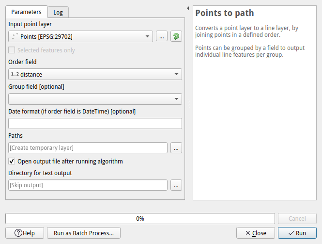
To convert the points to a line, I used the Points to path processing tool, and used the distance column (created by the previous tool) for the “order field” parameter.
Generating the data
A this point, if it is not the case yet, my profile line (the one I generated from points) and my DEM should be in a projected coordinate system. This is to avoid unit problems in our data. I used the Tananarive (Paris) / Laborde Grid approximation (EPSG 29702), a commonly used projection for Madagascar.
My next step is to generate a profile data from these in qProf, which can be called through the Plugins menu in QGIS’s main menu. When the plugin is called, a new qProf panel appears in QGIS’s user interface.
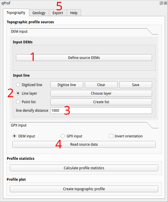
Under “Topography” tab, within “DEM input” this is what I did:
- under “Input DEMs” I selected my DEM
- under “Input line” I checked “Line layer” and chose my previously resampled road layer. For the “Line densify distance” I entered my sampling value, 1000 meters.
- I clicked on “Read source data”. At this point, qProf warns if the profile exceeds the 10 000 data points limit. This depends on the length of the line and the data points distance. For the sampling value I have chosen, I got 349 data points.
Under “Export” tab and within “Topographic profile data”, I exported the data as a CSV text for further editing and visualization in D3.js.
The data I obtained from qProf had these fields:
prof_id: As I only had one feature in my line layer, it had only one value, 1rec_id: Different for each point data, so 1 to 349 in my casex: X coordinatey: Y coordinatecds2d: 2D (horizontal) distance along the profilez: Z coordinate (elevation)cds3d: 3D (with elevation) distance along the profiledirslop: Directional slope along the profile (from Antananarivo to Toamasina) in degrees. Positive values indicate ascents and negative values indicate descents.
The CSV file can be downloaded from this link.
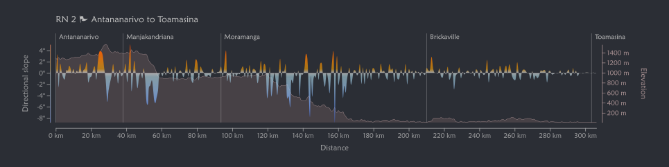
To get the graph at the beginning of this post, I simply plotted the Z coordinate (z) and the directional slope (dirslop) along the horizontal distance (cds2d), to get the elevation and directional slope graphs respectively. I put a live version of the graph with the 4 major roads of Madagascar on this page.
Going a little further
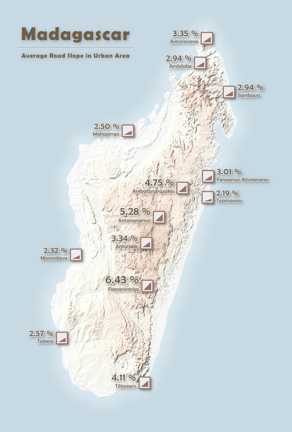
Using the same base but with a slightly different workflow, I could estimate the average street steepness in the major urban areas of Madagascar: